LLVM Obfuscator is an industry-grade obfuscator which we have encountered frequently in the past few years of CTFing. This blog post documents our work in understanding the design of the obfuscator itself, as well as any possible weaknesses in the implementations of the obfuscation passes. We use this work to automate the task of emitting cleaned and working binaries via Binary Ninja.
Introduction
The open source LLVM Obfuscator manifests as 3 relatively disjoint LLVM passes, each implementing some sort of obfuscation that obscures the CFG or arithmetic computation of the original program in some way.
Also note that, due to the fact that these passes operate over LLVM IR, it supports almost every architecture under the sun.
Information for each of the three passes can be found here:
These are simply the documentation pages maintained by the authors for each respective pass. However, if the documentation is deficient, the source is also an obvious ground truth.
Unfortunately, the llvm-obfuscator repo maintains multiple branches, one for each version of LLVM that that branch targets, with a clone of the entire LLVM repository, so it’s easy to get lost in the code. The passes for the 4.0 branch can be found here, in the lib/Transforms folder, as is customary for LLVM passes.
This blog post will focus on the control flow flattening pass, as we find it to be one of the most interesting passes in the LLVM Obfuscator ecosystem, as well as the most effective.
Control Flow Flattening
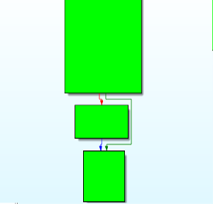
We can visualize the effects of the Control Flow Flattening pass as the following CFG transformation:
- Collect all of the original basic blocks in a CFG
- Lay them down flat “at the bottom” of the CFG, and remove all original edges
- Add some machinery which visits each basic block such that the semantics of the original program are preserved.
For illustration, we demonstrate two side-by-side images; on the left is a control flow graph generated by IDA 7.0 (the demo version is enough) for a program which is not obfuscated, and on the right is a control flow graph for the same program, compiled with llvm-obfuscator using only the Control-Flow Flattening pass.
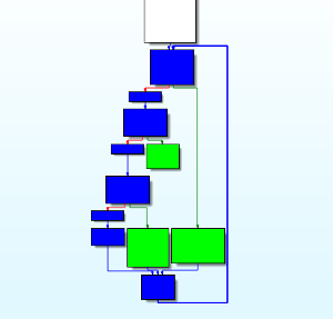
Here, green nodes denote the original basic blocks of the function, and blue nodes form the “machinery” which preserves the control flow semantics of the original program, mentioned before. At this point we name this machinery the backbone of the function, due to its shape in IDA (if you squint).
Another way we can visualize this CFG is by using IDA to group all of the blue basic blocks (i.e. the backbone) into a single node. This results in a CFG which appears closer to other control-flow flattening passes commonly seen in literature.
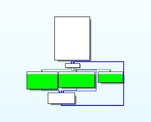
At this point, it’s clear that all control flow from the original program is completely obscured. It is also effective to note that this looks similar to a switch case statement, with each original basic block functioning as a case.
We can thus imagine that this code forms a state machine, with the end of each original basic block setting some state variable to target the next basic block in a semantics-preserving execution of the program, and with the backbone dispatching to the original basic block corresponding to some state.
Control Flow Flattening Weaknesses
From now on we’ll be using Binary Ninja for the analysis of the control flow flattening pass. This decision comes from certain features present in Binary Ninja that aren’t present in IDA in any usable form:
- Medium-level IL
- SSA Form
- Value-set analysis
Determining the Backbone Blocks
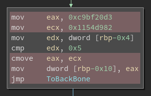
In order to understand the weaknesses in this particular implementation of the control flow flattening pass, we’ll need to discuss the backbone of a function emitted by the pass in more detail. We’ll use the following example:
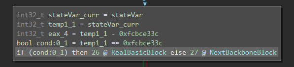
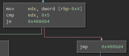
Shown above is a zoomed-in view of a node in the backbone of the previously obfuscated program. Pretty much each backbone node looks analogous; it reads the current state variable, and compares it to some case value. If it’s true, it executes an original basic block, or otherwise moves on to the next node in the backbone.
Now here is the first key weakness: given a definition of state_var, we can exploit the
fact that each backbone basic block contains at least one usage of the state variable, and
iterate through all uses of the variable provided by Binary Ninja’s medium-level IL to
collect each basic block.
def compute_backbone_map(bv, mlil, state_var):
    backbone = {}

    # Collect all mlil instructions where the state variable is used
    # `state_var` is the variable loaded in each backbone block to check the state,
    # either the state variable itself, or a pointer to it
    uses = mlil.get_var_uses(state_var)

    # Gather the blocks where the state is used
    blks = (b for idx in uses for b in mlil.basic_blocks if b.start <= idx < b.end)

    # In each of these blocks, find the value of the state
    for bb in blks:
        # Find the comparison
        cond_var = bb[-1].condition.src
        cmp_il = mlil[mlil.get_var_definitions(cond_var)[0]]

        # Pull out the state value
        state = cmp_il.src.right.constant
        backbone[state] = bv.get_basic_blocks_at(bb[0].address)[0]

    return backbone
Again, this algorithm will only work given at least one definition of the state variable. Luckily, the first basic block generally contains the first definition of the state variable, before it jumps right into the state machine, as seen below:
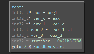
We thus target this definition of the state variable, as it is easy to find (via heuristics or via human interaction), and every backbone basic block that we’re targeting is reachable from it in the def-use and use-def chain graph.
Determining the Real Basic Blocks
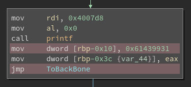
We can similarly expand examples of real basic blocks to glean some identifying features about them. In this case, a real basic block can either have a single successor or multiple successors (i.e. an unconditional jump or a conditional jump with a fall through). A real basic block with an unconditional jump looks something like below:
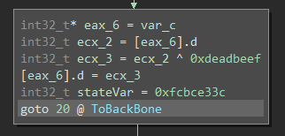
As we can see, we write a constant to the state variable, and return to dispatch. This
means that the next real basic block we’re taking corresponds to the case 0xfcbce33c. A
real basic block with multiple successors is slightly more interesting, as the cmov gets
expanded into multiple basic blocks in the MLIL view:
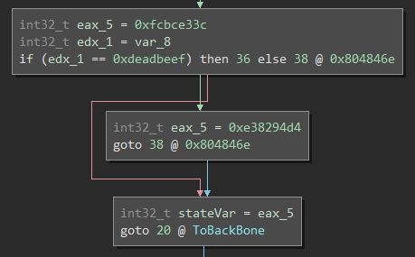
Here, we’re transforming the conditional from the original program into one which sets the state variable to the appropriate constant. In other words, the original source probably contained something of the form:
if (var == 0xdeadbeef) {
  // ...
}
But this has effectively been transformed into
state_var = var == 0xdeadbeef ?
  0xe38294d4 :
  0xfcbce33c;
Although this transformation is interesting, our end goal is to find all basic blocks which are present in the original program. In order to do this, we note one more key weakness in LLVM-Obfuscator: all original assembly basic blocks contain at least one definition of the state variable, similar to the entry basic block.
At first glance, it seems we’d need to perform a recursive depth-first search on the
def-use graph, though our task is in fact a lot easier. In the previous section we
were looking for all usages of state_var, though here we’re looking only in the
top-level:
## this gets all definitions of state_var, and
## we treat all such instructions as being in
## a real basic block
real = mlil.get_var_definitions(state_var)
real = itemgetter(*real)(mlil)
Each of these top-level definitions to state_var are treated as coming from an original
basic block, including the entry basic block. As we’ll see in the next section, this works
quite well when it comes time to emit a cleaned binary.
Recovering the CFG
At this point we have almost all the information to rebuild the control flow graph. As a refresher, we can currently compute the following information about an OLLVM-obfuscated binary:
- All the original basic blocks
- The mapping from state variables to original basic blocks
The last piece of the missing puzzle is actually determining the outgoing state on exit of a basic block. To accomplish this, we may hook into a powerful feature of Binary Ninja, Value-Set Analysis, an abstract interpretation technique which computes a precise approximation of all values which could potentially be held in a register or in a memory a-loc.
As mentioned before, in the case of an unconditional jump state_var is set to a
constant. This is easy enough to pick up given a new definition of state_var:
def resolve_cfg_link(bv, mlil, il, backbone):
    # il refers to a definition of the state_var
    bb = bv.get_basic_blocks_at(il.address)[0]

    # Unconditional jumps will set the state to a constant
    if il.src.operation == MediumLevelILOperation.MLIL_CONST:
        return CFGLink(bb, backbone[il.src.constant], def_il=il)
    # ...
Dealing with conditional jumps is a little trickier. The goal now is to determine which of two possible outgoing states is the false branch, and which is the true branch. For this, we utilize the SSA form of the medium-level IL that we’ve already been looking at.
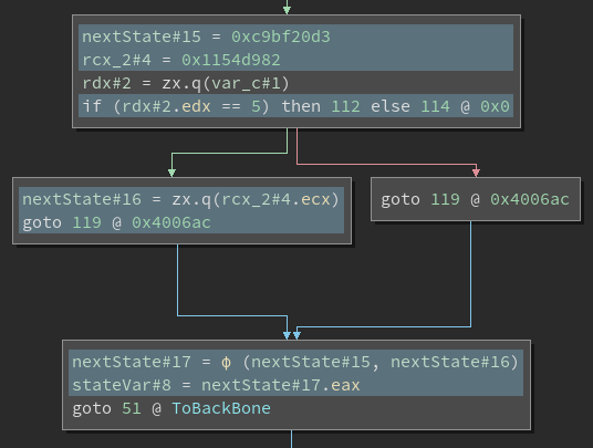
This shows an example of a block with two outgoing states in SSA form. The instructions that influence the selection of the next state have been highlighted here. We can better understand which state to choose by looking at the corresponding LLVM IR that produces this selection.
%next_state = select i1 %original_condition, i32 %true_branch, i32 %false_branch
store i32 %next_state, i32* %state
When compiled, this ends up having the general logic of:
- Lazily set
%next_stateto%false_branch - If
%original_conditionevaluates to1, overwrite%next_statewith%true_branch - set the new
%state
Looking back at the SSA-MLIL above, we can see that in the phi node, we are
choosing between two versions of the same nextState variable, each with their own
version numbers indicating which was defined first. Following the select logic, we take
the earliest version as the false state, and the other as true. Finally, taking advantage
of Binary Ninja’s value-set analysis, we can get the original values of the two instances
of nextState.
    # ...
    # Conditional jumps choose between two values
    else:
        # Go into SSA to figure out which state is the false branch
        # Get the phi for the state variable at this point
        phi = get_ssa_def(mlil, il.ssa_form.src.src)
        assert phi.operation == MediumLevelILOperation.MLIL_VAR_PHI

        # The cmov (select) will only ever replace the default value (false)
        # with another if the condition passes (true)
        # So all we need to do is take the earliest version of the SSA var
        # as the false state
        f_def, t_def = sorted(phi.src, key=lambda var: var.version)

        # There will always be one possible value here
        false_state = get_ssa_def(mlil, f_def).src.possible_values.value
        true_state  = get_ssa_def(mlil, t_def).src.possible_values.value

        return CFGLink(bb, backbone[true_state], backbone[false_state], il)
The API is currently a little awkward, but works immediately to get all possible values out of the assignment to the state variable at the end of an original basic block. Altogether, the core logic of our final script looks something like the following:
def deflatten_cfg(func, mlil, addr):
    state_var = func.get_low_level_il_at(addr).medium_level_il.dest
    backbone = compute_backbone_map(bv, mlil, state_var)
    original = compute_original_blocks(bv, mlil, state_var)
    CFG = [resolve_cfg_link(bv, mlil, il, backbone) for il in original]
    print "[+] Computed original CFG"
    pprint(CFG)

"""
[+] Computed original CFG
[<C Link: <block: x86_64@0x4006e7-0x400700> => T: <block: x86_64@0x400700-0x400720>,
                                               F: <block: x86_64@0x400735-0x400741>>,
 <U Link: <block: x86_64@0x4006d4-0x4006e7> => <block: x86_64@0x4006e7-0x400700>>,
 <U Link: <block: x86_64@0x400700-0x400720> => <block: x86_64@0x400720-0x400735>>,
 <U Link: <block: x86_64@0x4006b4-0x4006d4> => <block: x86_64@0x400741-0x400749>>,
 <U Link: <block: x86_64@0x400735-0x400741> => <block: x86_64@0x400741-0x400749>>,
 <C Link: <block: x86_64@0x400699-0x4006b4> => T: <block: x86_64@0x4006b4-0x4006d4>,
                                               F: <block: x86_64@0x4006d4-0x4006e7>>,
 <U Link: <block: x86_64@0x400720-0x400735> => <block: x86_64@0x4006e7-0x400700>>]
"""
Rebuilding Cleaned and Working Binaries
Unfortunately, patching programmatically is still a chore in Binary Ninja, though no other binary analysis framework seems to offer it either. At this point we’ve computed the original CFG of the program, all that’s left is to patch the original blocks so they jump to the next correct block(s) in the CFG, skipping the backbone.
Creating Code Caves
In each of the original basic blocks, some instructions were inserted for updating the state variable in order to maintain the original flow of the program. Now that the flattening machinery is being removed, we can remove these dead instructions to make room for our own that fix the CFG. We can remove the following from all original blocks:
- The current terminator. This is going to be replaced anyway, since no blocks should be going to backbone anymore.
- The instruction that updates the state variable
- All instructions in the def-use chain that determines the next state
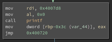
We can visualize the result of these removals with a few examples. First, we look at the dead instructions in a block with an unconditional jump. There is no def-use chain to follow here, so not much change is involved.
All of the instructions highlighted in red here were added by the flattening pass and can be removed. In a block with a conditional jump, there are few more instructions that can be removed:
Removing these instructions leaves more than enough room for our own patches, while cleaning up dead code left by the flattening pass as a bonus. In both cases, we make note of the instructions that can be removed and move on to the next step.
Fixing Control Flow
Now that we have room for a few new instructions in each original block, we can restore the original CFG of the program. This is as simple as inserting jumps to the correct blocks at the end of each original block. For a block with an unconditional jump, we only need to add a single instruction:
jmp next_block
In blocks with a conditional jump, we first need to determine which Jcc instruction to
use in our patch. Earlier, we made the assumption that the CMOVcc inserted by the
flattening pass always overwrites the false state with the true state. We know that the
flattening pass preserved the control flow of the original program using this CMOVcc,
so we can simply trust whatever condition it’s already using, and use that in our patch.
So, for example, if the flattened program used a cmovne, we can replace it with a jne,
and as long as we aren’t switching the true/false branches in the process the control
flow will be preserved. The final patch then looks like:
; cc is the condition used in the CMOVcc
jcc true_branch
jmp false_branch
With all of this defined, the patching process is simple. For each of the original basic blocks, we do the following:
- Re-emit a copy of the block with all the dead instructions omitted
- Append the jumps to the end of the block
- Pad to the length of the unmodified block with
nop
After applying this, we end up with the following results for a block with an unconditional jump (patched block on the right):
And for a block with a conditional jump:
At this point the original CFG of the program has been completely restored.
Final cleanup
After patching, the backbone is no longer reachable by anything in the CFG, so the entire
thing is now dead code and can be replaced with nops. This step is not necessary, but
disassembly tools that automatically run a linear sweep (i.e. IDA) will pick up the jumps
in the backbone and display it along with the fixed CFG. By replacing everything with
nops, we clean up the resulting CFG a little. We already computed the full backbone
earlier in this process, so it’s trivial to go through the blocks and nop them all out.
Results
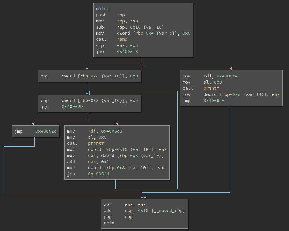
To show the effectiveness of the deflattening, let’s look at how it deobfuscates a test
program. Here is the original CFG of main, which is the end goal:
Here is the same function after applying control flow flattening:
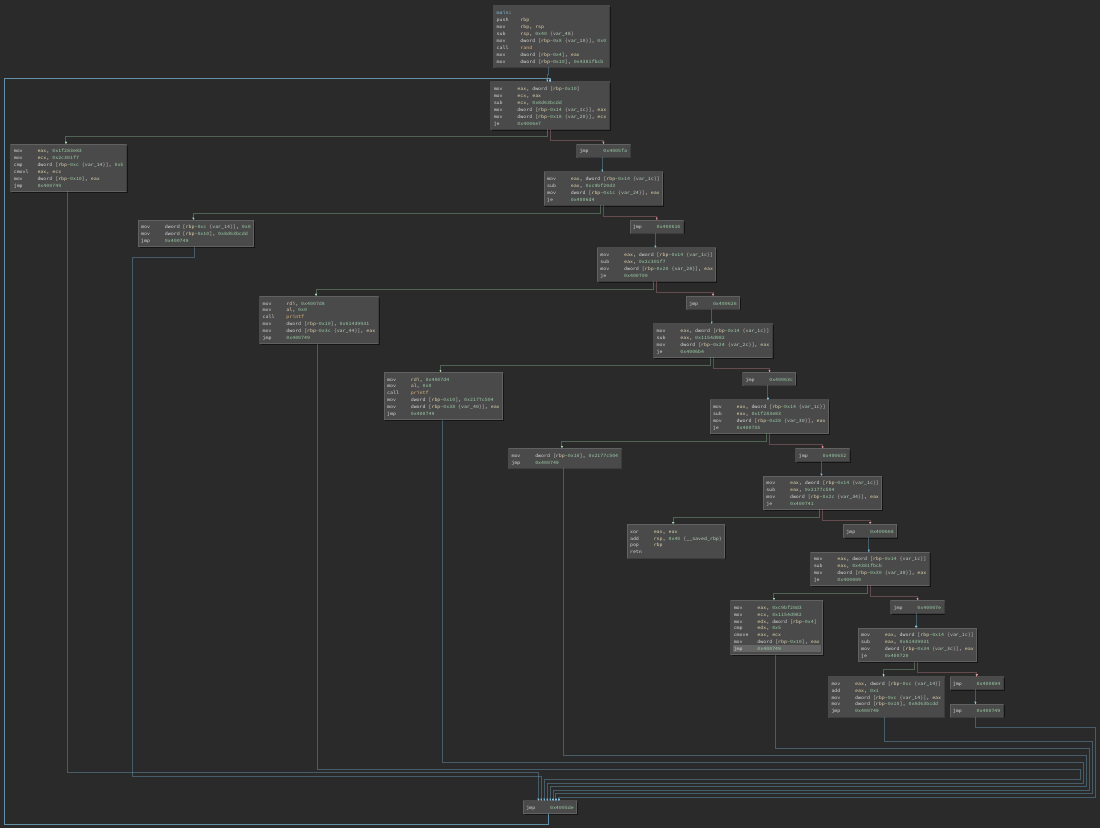
Here we can see the backbone running down the right side of the graph, with all the original blocks laid out on the left side.
Finally, here is the CFG after running the deobfuscator:
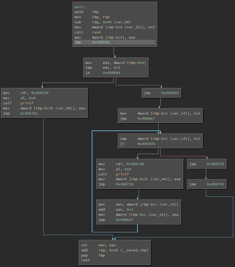
The recovered CFG comes very close to the original, with a few key differences:
- Some of the blocks were split by the flattening pass, and remain split in the deobfuscated function
- There are quite a few
jmps inserted around the CFG to connect blocks together
Both of these issues can’t be fixed without dealing with relocating all of the blocks in the function, which is a much harder problem to solve.
Using the Plugin
The source for this plugin is available on github. You can install it by cloning the repository to Binary Ninja’s plugin directory.
The steps to deobfuscate a flattened function are:
- Select any instruction that updates the state variable
- Run the deflattening plugin
The following clip demonstrates how to do this: